
I have been in contact with the National Hurricane Center with regards to the rouge wave theory as I posted yesterday, (The Story of the Sailing Vessel Sean Seamour II). This morning I received a reply. The NHC is assembling a report on the damages caused by Subtropical Storm Andrea which should be forthcoming shortly. The NHC is also taking a look at the rogue wave report and should be back to me in a couple of days.
I have also been in contact with scientists at the Great Lakes Environmental Research Laboratory (GLERL) who are studying rogue and freak waves and I expect to hear back from them shortly as well. The following paper was sent to me by Jamie Rhome of the National Hurricane Center. Its a must read for all mariners.
Maintaining Watch
RS
Expecting the Unexpected Wave: How the National Weather Service Marine Forecasts Compare to Observed Seas
Robbie Berg and Jamie R. Rhome, Tropical Analysis and Forecast Branch, NOAA/Tropical Prediction Center/National Hurricane CenterIntroduction
Marine forecasts issued by the National Weather Service (NWS) provide the sea state in terms of the significant wave height (Hs). This value is defined as the average of the highest 1/3 of the waves observed in a wave field. In other words, if a mariner were to observe the passage of 100 individual waves past a given point, the significant wave height would be the average height of the highest 33 waves. The concept of significant wave height was derived during a project to forecast ocean wave heights and wave periods during World War II (Stewart 2005). The Scripps Institute of Oceanography has shown that observed wave heights correspond to the average of the highest 20-40% of the waves, and the significant wave height has evolved to become the highest 1/3 of the waves (Wiegel 1964).
The significant wave height tends to be the height of the waves that is most readily observed by the human eye (WMO 1998). But how does this value compare to the average height of all the observed waves, or the highest wave one might encounter? Unfortunately, misunderstanding of the meaning of significant wave height often leads to improper interpretation of the NWS marine forecasts. Additionally, confusion surrounding the proper measurement of significant wave height leads to subjective and widely varying wave height reports from ships since every mariner would most likely report different wave height values for a given sea state. This is often exacerbated by the fact that observations are dependent on the size of the vessel and the height at which the observation is taken. For example, observations of significant wave heights taken on the main deck of a large ship 80-100 feet above the water often cause the waves to appear smaller than reality. Similarly, a small vessel encountering rough seas may overestimate significant wave height or report only the highest individual waves (WMO 1998). This subjectivity results in vastly different reports of significant wave height from adjacent ships, forcing marine forecasters to speculate as to which report best represents the prevailing sea state. Accurate sea height estimates are critical to the accuracy of the NWS marine program. Accordingly, this paper seeks to provide additional insight into the term significant wave height and its relationship to other wave statistics.
Significant Wave Heights
If a NWS forecast calls for seas 12 to 14 feet, exactly how will the wave field look to a mariner? To better understand what the significant wave height is and what it means to the mariner, we need to turn to statistics and the concept of distributions. Most people are aware of statistical distributions and probably don't even know it. The most common distribution used in real life is the normal, or Gaussian distribution (Figure 1A), which is more commonly referred to as the bell curve because of its shape (Wilks 1995). This distribution is quite good at describing phenomena in which most elements in a group are clustered near an average value with an equal number of elements being greater and less than this average value. Examples include the high temperature in a city for a given day, the weight of babies born at a hospital, or the height of students in a college oceanography class.
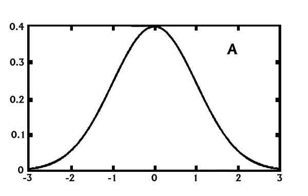 | 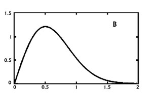 |
Figure 1. Generalized normal (a) and Rayleigh (b) distributions. | |
Wave heights in the ocean are usually modeled according to another statistical distribution called the Rayleigh distribution (Figure 1B). This distribution also has an average value, but in this case most elements are clustered toward lower values, with only a few exceptionally large values. The Rayleigh distribution does not exhibit symmetry like the normal distribution (Wilks 1995).
Several different wave statistics useful to the mariner can be inferred from the Rayleigh distribution. For example, the highest point of the distribution can be thought of as the most frequent wave height observed in the wave field. Roughly speaking, the most frequent wave height Hf is approximately half the value of the significant wave height (see Appendix). Similarly, the average wave height, which will be slightly larger than the most frequent wave, is estimated to be about 5/8 the value of the significant wave height (see Appendix).
Several recent marine incidents have highlighted the importance of knowing the height of the largest wave that can be expected for a given wave forecast. Since the Rayleigh distribution actually goes to infinity to the right of its peak, a wave is theoretically not bounded by a limiting height. This is where the Rayleigh assumption breaks down. Luckily, however, the highest waves can still be estimated through a combination of several methods. For example, it can be shown that 10% of the waves have a height greater than 1.074 times the significant wave height, and the average height of those highest 10% of the waves is approximately 1.272 times the significant wave height (see Appendix). Table 1 shows the relationship between the multiple wave statistics for several common significant wave height forecast values.
| Significant Wave Height (Hs) | Most Frequent Wave Height (Hf) | Average Wave Height ( ) | Average of Highest 10% of Waves ( ) |
| 4 | 2 | 2.5 | 5 |
| 8 | 4 | 5 | 10 |
| 10 | 5 | 6 | 13 |
| 12 | 6 | 7.5 | 15 |
| 15 | 7.5 | 9 | 19 |
| 20 | 10 | 13 | 25 |
| Wave conditions at NDBC Buoy 42040 during Hurricane Ivan | |||
| 52.4 | 26.1 | 32.8 | 66.7 |
Table 1. Relationship between selected National Weather Service forecast wave heights (significant wave height in feet) and other parameters such as most frequent wave height, average wave height, and average height of the highest 10% of waves (also in feet.) The most frequent wave height, average wave height, and average of the highest 10% of waves at Buoy 42040 during Hurricane Ivan are calculated from the theoretical Rayleigh distribution for the observed significant wave height of 52.4 feet.
In a somewhat tedious process, the above information can be combined with the parameters of the Rayleigh distribution to arrive at a relationship between the significant wave height and the highest expected waves (see Appendix). As an example, assume that the significant wave height in an area is 10 feet. One out of every 100 waves (or 1% of the waves) will have a height greater than about 16 feet. One out of every 1000 waves (or 0.1% of the waves) will have a height greater than about 19 feet. A common rule of thumb often utilized is that the highest expected wave is equal to twice the significant wave height. This kind of height would be observed in about 1 out of every 3000 waves. Incidentally, if an average wave period is known, the frequency of observing the highest expected wave can be obtained by multiplying 3000, or any other number of waves, by the wave period. If the average wave period is 10 seconds, then a wave two times as high as the significant wave height will be observed on average every 30,000 seconds, or about 8.3 hours. In reality, wave height is limited by wave steepness: deep water waves (those in an area where the ocean depth is greater than half the wavelength) begin to break when their height to length ratio exceeds 1/7 (see Appendix).
Here's an example to put all this into context. On September 15, 2004, Hurricane Ivan was racing northward across the Gulf of Mexico towards the Alabama and Florida coastline with strong 115 kts winds that were producing extremely large waves. The Tropical Analysis and Forecast Branch (TAFB) at the Tropical Prediction Center/National Hurricane Center predicted seas (significant wave heights) as high as 55 ft the morning before the hurricane moved into the northern Gulf of Mexico, and this forecast verified quite well with a significant wave height of 52.4 ft reported at NDBC buoy 42040 at 8:00 p.m. as the center of Ivan passed overhead. But not every wave that passed the buoy had a height of 52 feet, so what was the character of the actual wave field during the hurricane?
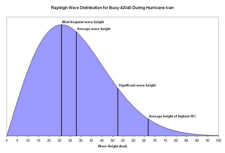 |
Figure 2. Theoretical Rayleigh distribution of the wave heights at Buoy 42040 at 8:00 p.m. September 15, 2004 as Hurricane Ivan was passing overhead. |
A significant wave height of 52 feet seems quite large, but realistically a sizeable portion of the actual waves during the hurricane did not attain that height. The most frequent wave height, according to the Rayleigh distribution, was about 26 feet - still an imposing and dangerous wave for a mariner out at sea. A few waves did build higher than the significant wave height, with the average of the highest 10% of the waves being around 67 feet! Figure 2 shows the theoretical distribution of the wave heights at Buoy 42040 as Hurricane Ivan was passing overhead, and the last row in Table 1 gives the calculated values from the distribution.
There is a limit on the highest wave that would be expected. The average wave period reported by the buoy at the same time as the report of the maximum wave height was about 12 seconds. Therefore, a wave with a 12 second period (which incidentally would have a wavelength of 735 feet), would break when its wave height exceeded 105 feet. Individual waves with shorter periods would break at much shorter wave heights. Based on the rule of thumb for the highest expected wave, a significant wave height of 52 feet could yield a wave of about 104 feet, which lies within the possible range of wave heights given the breaking wave height.
Conclusion
The NWS marine forecasts provided by the Tropical Prediction Center, Ocean Prediction Center, and coastal Weather Forecast Offices convey important wave field information that goes beyond just the expected significant wave height. Other useful wave parameters, such as the most frequent wave and highest expected waves, can be derived that can go into making important decisions regarding safe marine operations. Estimations of the highest expected wave height are especially important in extreme weather events and can be beneficial when trying to avoid large and occasionally devastating storm-generated waves. So, don't be caught off guard by a 26 foot wave the next time the NWS marine forecast reads "SEAS 12 TO 15 FEET"!
References
Stewart, Robert H., 2005: Introduction to Physical Oceanography.
(Available at http://oceanworld.tamu.edu/resources/ocng_textbook/contents.html)
Wiegel, R. L., 1964: Oceanographical Engineering. Prentice Hall, Englewood, NJ.
Wilks, D. S., 1995: Statistical Methods in the Atmospheric Sciences. Academic Press, San Diego, CA, 467 pp.
WMO, 1998: Guide to Wave Analysis and Forecasting. WMO No.-702, Second Edition, 168 pp. (Available from http://www.wmo.ch/index-en.html).
Biography
Robbie Berg has worked as a forecaster in the Tropical Analysis and Forecast Branch of the Tropical Prediction Center/National Hurricane Center since June 2002. He received two B.S. degrees in meteorology and marine sciences from North Carolina State University and is currently pursuing a M.S. degree in meteorology from the University of Miami. Previous work experience includes hurricane research at the NOAA Environmental Technology Laboratory in Boulder, Colorado.
Jamie Rhome has worked as a forecaster in the Tropical Analysis and Forecast Branch of the Tropical Prediction Center/National Hurricane Center since September 1999. He received his B.S. and M.S. degrees in meteorology from North Carolina State University. Previous work experience includes the United States Environmental Protection Agency and the State Climate Office of North Carolina. In addition to his professional experience in marine meteorology, Jamie is an avid offshore fisherman.
Acknowledgments
The authors wish to thank Eric Holweg, Dr. Rick Knabb, Alison Krautkramer, and Daniel Brown for their constructive comments and suggestions on this paper.


![[Valid RSS]](valid-rss.png "Validate my RSS feed")